Multiple Runs on a Local Computer
Mission Setup
Running single simulations is helpful for directly observing autonomous behaviors. However, if you want to statistically compare various algorithms, you will need to generate hundreds, thousands, or millions of runs. SCRIMMAGE ships with scripts that generate scenarios with different initial conditions based on an initial scenario file and then runs the scenarios on your local machine in parallel. The following describes the workflow for generating scenarios from a base scenario, executing the runs on your local machine in parallel, and then analyzing the results with SCRIMMAGE’s tools.
In this example, we will be setting up an experiment to determine the
effectiveness of the collision avoidance behavior provided by Motor Schemas. To
accomplish this we will first setup a team to serve as a control group, where
the control group is not using collision avoidance. The team without collision
avoidance will be split into two groups, each initially heading towards each
other. Using the variance_x, variance_y, and variance_z XML tags,
we can vary how far the entities will be generated around the entity’s x,
y, and z position tags. The control group will use the Straight
Autonomy plugin, which simply drives the entity in the forward direction based
on its initial heading.
The second team will use the MotorSchemas Autonomy plugin. This autonomy
plugin attempts to drive the entity in the forward direction based on its
initial heading, but it will also try to avoid other entities that enter its
sphere_of_influence. The second team will also be split into two groups and
will initially point at each other, but they will be offset from the control
group, so that they do not interact.
This SCRIMMAGE mission is provided by the straight-vs-motorschemas.xml
mission, which is located in the SCRIMMAGE core missions directory. Let’s take
a look at the important aspects of this mission.
<!-- ========================== TEAM 1 ========================= -->
<!--                   No Collision Avoidance                    -->
<entity>
  <team_id>1</team_id>
  <count>20</count>
  <autonomy>Straight</autonomy>
  ...
</entity>

<entity>
  <team_id>1</team_id>
  <count>20</count>
  <autonomy>Straight</autonomy>
  ...
</entity>

<!-- ========================== TEAM 2 ========================= -->
<!--          Running MotorSchemas with Collision Avoidance      -->
<entity>
  <team_id>2</team_id>
  <count>20</count>
  <autonomy sphere_of_influence="50">MotorSchemas</autonomy>
  ...
</entity>

<entity>
  <team_id>2</team_id>
  <count>20</count>
  <autonomy sphere_of_influence="50">MotorSchemas</autonomy>
  ...
</entity>
First of all, the mission contains four entity’s: two entities for team #1
running the Straight Autonomy plugin and two entities for team #2 running
the MotorSchemas Autonomy plugin. Also, each entity XML block will actually
generate 20 entities. This is a key feature of SCRIMMAGE that makes it more
versatile at developing swarm-based algorithms compared to other robotics
simulators. Also, note that the team #2 autonomy tag sets the
sphere_of_influence tag to 50. This allows a higher-level mission file to
override sub-XML file parameters. If you open up the MotorSchemas.xml file in
the SCRIMMAGE core project, you will find:
<sphere_of_influence>10</sphere_of_influence>
By setting the sphere_of_influence in the autonomy tag’s attribute, we
change the value from 10 to 50. This can be accomplished for arbitrary
parameters in SCRIMMAGE XML files.
Run Single Mission
Let’s execute a single simulation run to ensure that our initial conditions are
correct. We can run the scrimmage executable from anywhere on the system as
long as we provide a relative or absolute path to the mission file.
$ cd ~/scrimmage/scrimmage
$ scrimmage ./missions/straight-vs-motorschemas.xml
Click on the SCRIMMAGE viewer window to bring it into focus. You can use your mouse and keyboard to navigate around the environment as described in Viewer Controls (You will have to hit the ‘a’ key to cycle between camera types). You should see four groups of aircraft in the SCRIMMAGE environment. Type ‘b’ to start the simulation. After the simulation is complete, the SimpleCollisionMetrics will print out a report of the events it recorded and the weighted score. For example, the following output may be generated:
================================================================================
SimpleCollisionMetrics
================================================================================
Team ID: 1    (Survived round)
Score: -6
Entity Count: 60
Total Flight Time: 5557.4
Total Normalized Flight Time: 55.574
Non-Team Collisions: 0
Team Collisions: 6
Ground Collisions: 0
----------------------------------------------------------------------
Team ID: 2    (Survived round)
Score: 0
Entity Count: 20
Total Flight Time: 2000
Total Normalized Flight Time: 20
Non-Team Collisions: 0
Team Collisions: 0
Ground Collisions: 0
----------------------------------------------------------------------
================================================================================
Overall Scores
================================================================================
Team ID: 1
Score: -6
--------------------------------------------------------------------------------
Team ID: 2
Score: 0
--------------------------------------------------------------------------------
Simulation Complete
From this report, you can see that team #1 (the team without collision avoidance) had six team collisions and that team #2 (the team with collision avoidance) had zero team collisions. The SimpleCollisionMetrics plugin uses the weights defined in SimpleCollisionMetrics.xml to compute the final score. Thus, with the weights:
<!-- weights for scoring function -->
<flight_time_w>0.0</flight_time_w>
<team_collisions_w>-1.0</team_collisions_w>
<non_team_collisions_w>-1.0</non_team_collisions_w>
team #1 was assigned a score of -6, while team #2 was assigned a score
of 0. Thus, for this example, the team with collision avoidance performed
better. The metrics are also saved to a CSV file called summary.csv in the
output log directory. In this case, the file can be found at:
~/.scrimmage/logs/2017-07-25_16-15-05/summary.csv.
Multiple Runs in Parallel
Before running multiple scenarios in parallel, you will need to be sure you have followed the install with Python Bindings then install some additional Python packages:
$ sudo apt-get install python-pip python-scipy python-pandas parallel
$ sudo pip install pyDOE tqdm
We will now use one of SCRIMMAGE’s tools, run_experiments.py, to execute
100 simulation runs of this same scenario (7 instances allowed in parallel)
$ cd ~/scrimmage/scrimmage/scripts
$ ./run_experiments.py -t 100 -m ../missions/straight-vs-motorschemas.xml -r ../config/ranges/batch-ranges.xml -p 7
Since my machine has eight cores, I allow seven SCRIMMAGE instances to run in
parallel at a time to prevent system lockup. After the 100 simulations finish
executing, you should have a new timestamped folder in ~/.scrimmage/experiments
and an additional 100 timestamped log folders under that. The
aggregate-runs program is used to read the summary.csv files in each log
directory, tally the wins for each team, and display the results. Let’s
aggregate the results by providing the directory that holds all the results to
the aggregate-runs program:
$ aggregate-runs ~/.scrimmage/experiments/{new_timestamped_folder}
This should produce a terminal output that looks something like this
Aggregating 100 runs.
[======================================================================] 100 %
Total time to process log files: 0.002509
-----------------------------------------------------
Team ID         Wins            Draws           Total
2               100             0               100
To see other inputs to run_experiments.py, view its command line help with
the -h flag.
Playback Scenarios
Sometimes your results might contain outliers that you want to look at
closer. For example, what if there was a mission where team #1 outperformed
team #2? You could use the filter-runs program to playback the scenario
that contains the outlier. Execute filter-runs by providing it with the log
directory:
$ filter-runs ~/.scrimmage/experiments/{new_timestamped_folder}
Now you can select the type of outcome to playback:
====================================================
Choose an outcome number:
----------------------------------------------------
Number          Name            Count
----------------------------------------------------
[0]             team_2          100
>>
In this case, there were no outliers and team #2 always won. But, we can
playback the scenarios where team #2 won by entering 0 and hitting
[ENTER]. This will open the SCRIMMAGE viewer and playback the
simulation. Also, some information about the simulation is displayed to the
screen:
Playing back: team_2
Mission: ~/.scrimmage/experiments/{new_timestamped_folder}/{timestamp}_job_0_task_50
Frames parsed: 502
Playback Complete
====================================
Choose an option:
(r)eplay
(n)ext
(q)uit
The user can then use the r, n, and q keys to replay the same
scenario, move to the next scenario, or quit the filter-runs program,
respectively. The user can also playback specific scenarios by providing the
log directory of a specific scenario to the scrimmage-playback program:
$ scrimmage-playback ~/.scrimmage/experiments/{new_timestamped_folder}/{timestamp}_job_0_task_50
Varying Initial Conditions
SCRIMMAGE also has the ability to vary initial conditions in the SCRIMMAGE
mission file with the use of a “ranges” file. Let’s take a look at the example
mission file located at /path/to/scrimmage/missions/batch-example-mission.xml.
<autonomy show_shapes="true" max_speed="${max_speed=25}" behaviors="
  [ AvoidEntityMS show_shapes='true' gain='${MS_gain=1.0}' sphere_of_influence='10' minimum_range='2' ]
   [ MoveToGoalMS gain='1.0' show_shapes='true' use_initial_heading='true' goal='200,200,-100']"
          >MotorSchemas</autonomy>
In this example we can see that we have created two variables - max_speed and
MS_gain. These variables are enclosed by braces and have a dollar sign at the
beginning. The basic format is ${var_name=value}. You must also provide a
default value for the variables to the right of the equal sign. In this
example, the default max_speed is 25, and the default gain is 1.0. Everything
from the $ to the } will become that variables value, so be sure to enclose the
expression in the proper quotations. Let’s now take a look at the ranges file,
/path/to/scrimmage/config/ranges/batch-ranges.xml.
<?xml version="1.0"?>
<?xml-stylesheet type="text/xsl" href="http://gtri.gatech.edu"?>
<ranges xmlns:xsi="http://www.w3.org/2001/XMLSchema-instance"
    name="BatchExample">
    <MS_gain low="0" high="2" type="float"/>
    <max_speed low="15" high="25" type="float"/>
</ranges>
By providing the path of this ranges file to the run_experiments.py
script, SCRIMMAGE will vary the max_speed and gain for MoveToGoalMS for each entity
based on the low and high values specified in the ranges file.
Let’s execute 100 simulations again, but we’ll vary the initial conditions with the ranges file this time. Lets also name the mission this time:
$ cd ~/scrimmage/scrimmage/scripts
$ ./run_experiments.py -t 100 -m ../missions/batch-example-mission.xml \
  -p 7 -r ../config/ranges/batch-ranges.xml -n my_first_parameter_varying
This should output 100 timestamped folders to
~/.scrimmage/experiments/my_first_parameter_varying/ representing the files for each
individual run. In addition, it will output a params file for each run and a
batch_params.csv file showing all of the params for each file in one run.
Aggregating Multi-run Data
In your webbrowser, navigate to
https://nbviewer.jupyter.org/github/gtri/scrimmage/blob/master/scripts/BatchExample.ipynb
This is a python jupyter notebook showing a simple example of how to aggregate
data from this tutorial. In this example, we output all of the data on entity 1
per run into a single .csv file saved at
~/.scrimmage/experiments/my_first_parameter_varying/entity_1_data.csv.
You can run the aggregation of the data locally with either Jupyter Notebooks or with python script to produce the indicated csv file
$ sudo pip install statsmodels
$ python BatchExample.py
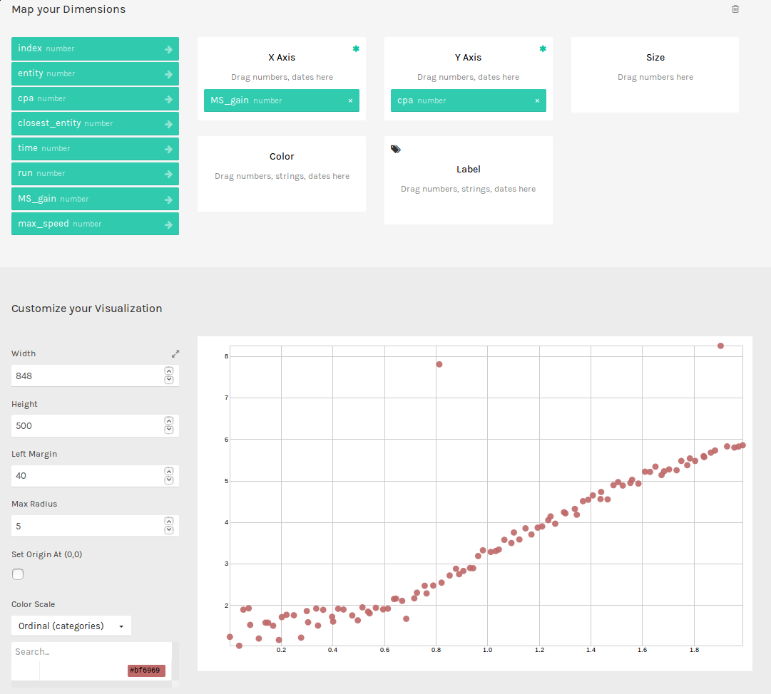
Basic Visualization
This .csv file that we just generated is formatted nicely to work with many
visualization tools. One tool that will allow you to quickly generate graphs is
RAW Graphs. Navigate to http://app.rawgraphs.io/. You will see a button that
allows you to upload a csv file. Upload
~/.scrimmage/experiments/my_first_parameter_varying/entity_1_data.csv. You
can then scroll down and quickly generate graphs for this data. An example
graph for this data is included below. This graph demonstrates an intuitive
result - increasing the gain on AvoidEntityMS causes the Closest Point of
Approach (CPA) to increase. RAW Graphs can also set up to run locally by
following the instructions on their github page:
https://github.com/densitydesign/raw/